|
|
 |
Klein polyhedra
Romanian translation of this webpage
I work in  , and in the lattice , and in the lattice  embedded in it.
Consider three planes with (not necessarily unit) normals embedded in it.
Consider three planes with (not necessarily unit) normals
 through the origin. Consider the octant defined by
 .
Now form the convex hull of the points of
(excluding the origin) contained in this octant.
This is the Klein polyhedron of the cubic form .
Now form the convex hull of the points of
(excluding the origin) contained in this octant.
This is the Klein polyhedron of the cubic form

Klein polyhedra are also known as Arnold sails or veils
(voiles in French). These were proposed over 100 years ago by Klein,
but have only become of interest again in the last 10 years.
To visualize a Klein polyhedron, we take a finite piece near the origin and flatten
the piece onto a plane to produce images such as in the next section.
More precisely, for each vertex point x in the convex hull, we let
 and
and

and plot  .
Thus .
Thus  , so by plotting any two
components we have full information.
(In a few cases I plot other coordinates of , so by plotting any two
components we have full information.
(In a few cases I plot other coordinates of  than 1 and 2 in order to compare with published results.)
These are joined by straight lines.
These lines would be curved if they were the true projections of the
edges of the convex hull, but the picture is clearer with straight lines.
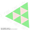
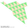
The black dots within faces are points of the convex hull which are not
boundary points of a face. The faces are coloured by type, in an attempt
to make the periodicity clear. Sometimes this colouring can go wrong at the edges.
than 1 and 2 in order to compare with published results.)
These are joined by straight lines.
These lines would be curved if they were the true projections of the
edges of the convex hull, but the picture is clearer with straight lines.
The black dots within faces are points of the convex hull which are not
boundary points of a face. The faces are coloured by type, in an attempt
to make the periodicity clear. Sometimes this colouring can go wrong at the edges.
The main point of interest is that the patterns are periodic iff the planes
are related to a totally real cubic number field. The exact relationship
is discussed in the papers of Lachaud and Korkina referenced below.
Aim
My main interest was the development of algorithms for constructing these
figures. There is an algorithm in the thesis of
J.-O. Moussafir
referenced below, but I didn't like this so much because it works with rational approximations to the planes, and I was interested in irrational planes. After a lot of experimentation with computing exactly the convex hull of very large sets of points with integral coordinates, I found I had best success with the
hull program
by Ken Clarkson.
Examples
Some of the examples are taken from the papers in the bibliography below.
For each example, I give the generating polynomial  of the cubic field
and a matrix whose columns
give the coefficients of the normal vectors.
In some cases I also give a (symmetric and unimodular if possible)
integral matrix m whose
characteristic polynomial is . In these cases we know that Korkina's
theorem (Thm 3.5 on page 135 of [Korkina 1995]) applies, so that the pattern
has two periods. of the cubic field
and a matrix whose columns
give the coefficients of the normal vectors.
In some cases I also give a (symmetric and unimodular if possible)
integral matrix m whose
characteristic polynomial is . In these cases we know that Korkina's
theorem (Thm 3.5 on page 135 of [Korkina 1995]) applies, so that the pattern
has two periods.
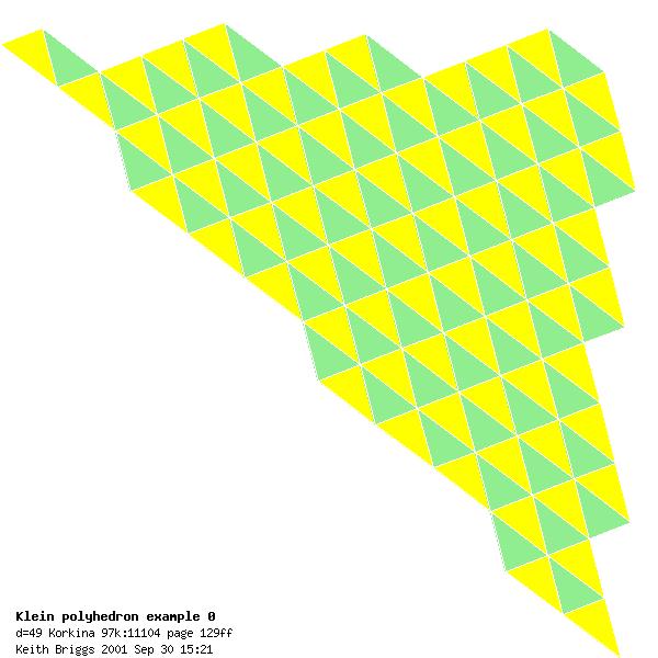
Example 0
Korkina MR97j:11032 pages 129ff
(MathSciNet lookup)
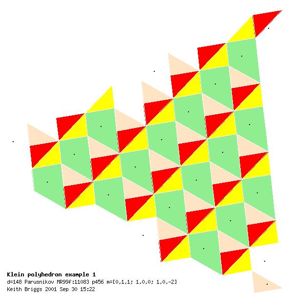
Example 1
Parusnikov MR99f:11083 page 456.
Plotted:  (Misprint in paper?) (Misprint in paper?)
|
Roots  of of 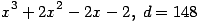 (3rd extremal Davenport form), (3rd extremal Davenport form), ![, m=[0,1,1; 1,0,0; 1,0,-2] ...(123.3)](eqn/klein-polyhedra_eqn_123_3.png)
|
Example 2
Parusnikov MR96a:11061 page 999
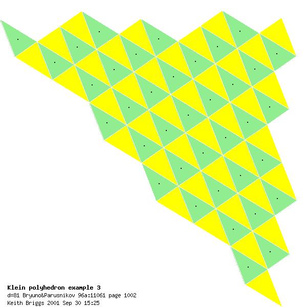
Example 3
Parusnikov MR96a:11061 page 1002
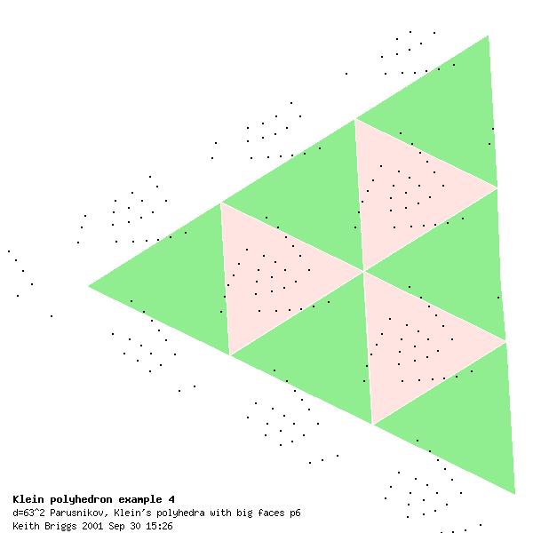
Example 4
Parusnikov, Klein's polyhedra with big faces, page 6
Plotted:
|
Roots of 
(4th extremal Davenport form)
|
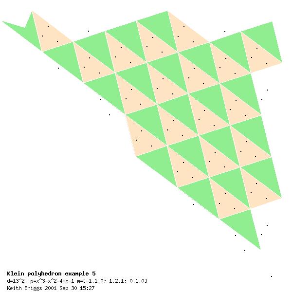
Example 5
This is the first of a series of examples (except example 10)
where we run through the
totally real cubic fields in order of discriminant as listed in Appendix B
of Cohen's book A course in computational algebraic number theory,
starting with discriminant 169. Until discriminant 961, an integral basis
is always given by  , where , where  is a root
of the defining polynomial.
Thus, unless otherwise stated, from now on the matrix is always of the
same form as this example. is a root
of the defining polynomial.
Thus, unless otherwise stated, from now on the matrix is always of the
same form as this example.
|
Roots of ![x^3-x^2-4x-1,\; d=13^2=169,\; m=[-1, 1, 0; 1, 2, 1; 0, 1, 0] ...(255.1)](eqn/klein-polyhedra_eqn_255_1.png)
|
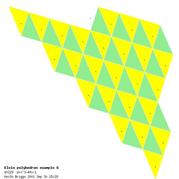
Example 6
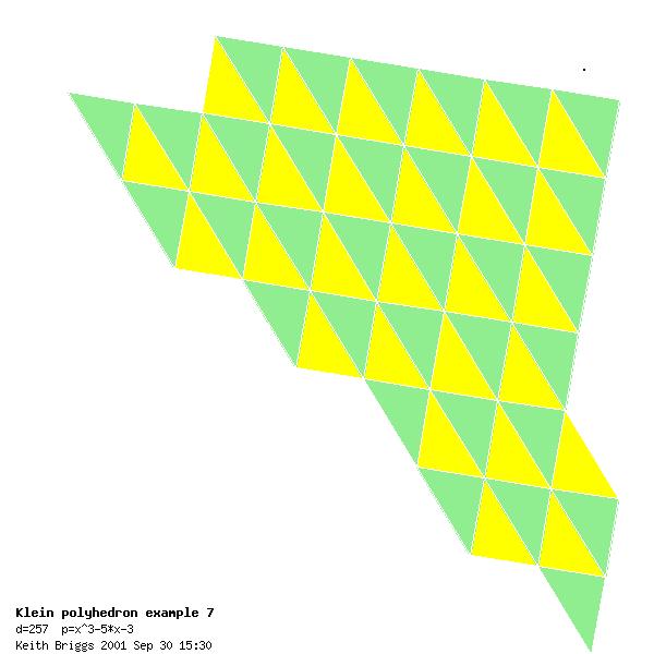
Example 7
Example 8
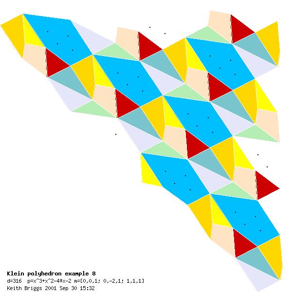
Example 9
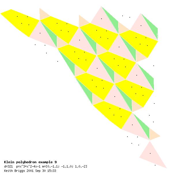
Example 10
Parusnikov, Klein's polyhedra for the fifth extremal cubic form, page 6.
Example 11
Example 12
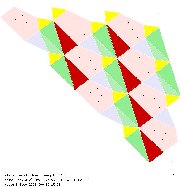
Example 13
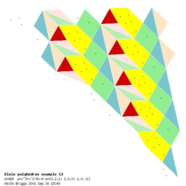
Example 14
Example 15
Example 16
Example 17
Example 18
Example 19
Example 20
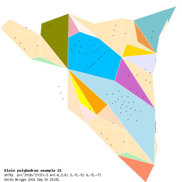
Example 21
Example 22
Example 23
Example 24
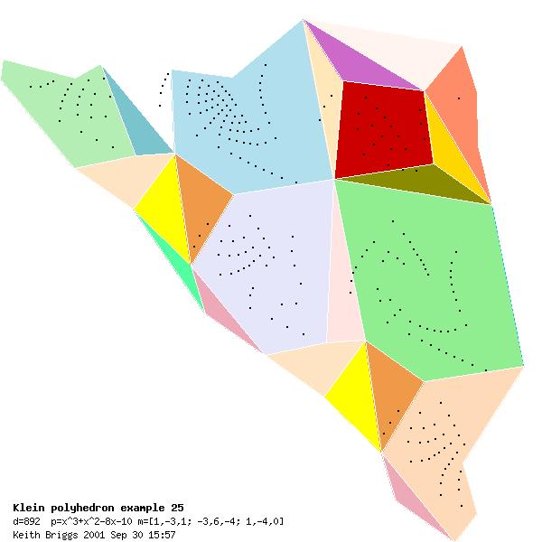
Example 25
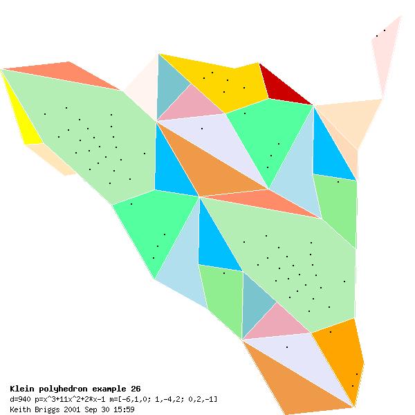
Example 26
Links
V. I. Arnold |
A. D. Bruno |
F. C. Klein |
J.-O. Moussafir
Bibliography
Some preprints are from the Keldysh Institute of the Russian Academy of Sciences, Moscow.
- [AO82]
- H. Appelgate and H. Onishi.
Periodic expansion of modules and its relation to units.
J. Num. Th., 15:283-294, 1982.
- [Arn98]
- V. I. Arnold.
Higher dimensional continued fractions.
Regular and chaotic dynamics, 3:10-17, 1998.
MR 2000h:11012.
- [BP94a]
- A. D. Bryuno and V. I. Parusnikov.
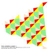
Klein polyhedra for two Davenport cubic forms.
Mat. Zametki, 56(4):9-27, 156, 1994.
- [BP94b]
- A. D. Bryuno and V. I. Parusnikov.
Klein polyhedrals for two cubic Davenport forms.
Mathematical notes, 56(3-4):9-27, 1994.
96a:11061.
- [BP97]
- A. D. Bryuno and V. I. Parusnikov.
Comparison of various generalizations of continued fractions.
Mathematical notes, 61:278-286, 1997.
(was Keldysh Institute of the RAS, preprint 52 of 1994).
- [Buc87]
- J. Buchmann.
On the computation of units and class numbers by a generalization of
Lagrange's algorithm.
J. Number Theory, 26:8-30, 1987.
- [Coh78]
- H. Cohn.
Formal ring of a cubic solid angle.
J. Num. Th., 10:135-150, 1978.
- [HP00]
- U. Halbritter and M. E. Pohst.
On lattice bases with special properties.
J. de Théorie des Nombres de Bordeaux, 12:437-453, 2000.
- [HW97]
- M. Henk and R. Weismantel.
Hilbert bases of cones and simultaneous Diophantine approximations and linear
Diophantine equations.
Technical Report SC 97-29, Konrad-Zuse-Zentrum für Informationstechnik
Berlin, Berlin, 1997.
- [HW01]
- M. Henk and R. Weismantel.
Diophantine approximations and integer points of cones.
Technical report, TU Wien, Wien, 2001.
to appear in Combinatorica.
- [Isl01]
- Iman Islim.
Sur les unités et les polyèdres de Klein en théorie algébrique des
nombres.
PhD thesis, Université de la Méditerranée Aix-Marseille II, Faculté des
Sciences de Luminy, 2001.
- [Kle95]
- F. Klein.
Ueber eine geometrische Auffassung der gewöhnliche
Kettenbruchentwicklung.
Nachr. Ges. Wiss. Göttingen Math-Phys. Kl., 3:357-359,
1895.
- [Kle96]
- F. Klein.
Sur une représentation géométrique du développement en fraction
continue ordinaire.
Nouv. Ann. Math., 15(3):327-331, 1896.
[Not pages 321-331 as often cited].
- [Kor94]
- E. Korkina.
La périodicité des fractions continues multidimensionelles.
C. R. Acad. Sci., 319:777-780, 1994.
MR 95j:11064.
- [Kor95]
- E. I. Korkina.
Two-dimensional continued fractions. The simplest examples.
Proc. Steklov Institute of Mathematics, 209:124-144, 1995.
MR 97k:11104.
- [Kor96]
- E. I. Korkina.
The simplest 2-dimensional continued fraction.
J. Math. Sci., 82(5):3680-3685, 1996.
- [KS]
- M. L. Kontsevich and Yu. M. Suhov.
A new approach to multidimensional continued fractions.
Cambridge University preprint, no date, c1998.
- [KS99]
- M. L. Kontsevich and Yu. M. Suhov.
Statistics of Klein polyhedra and multidimensional continued fractions.
Am. Math. Soc. Trans., 197:9-27, 1999.
- [Lac93]
- G. Lachaud.
Polyèdre d'Arnol'd et voile d'un cône simplicial: analogues du
théorème de Lagrange.
C. R. Acad. Sci. Paris, 317:711-716, 1993.
94m:11081.
- [Lac98a]
- G. Lachaud.
Klein polygons and geometric diagrams.
In Contemporary mathematics, volume 210, pages 365-372. 1998.
MR 99a:11086.
- [Lac98b]
- G. Lachaud.
Sails and Klein polyhedra.
In Contemporary mathematics, volume 210, pages 373-385. 1998.
MR 98k:11094.
- [Mou00]
- J.-O. Moussafir.
Voiles et Polyèdres de Klein: Géométrie, Algorithmes et
Statistiques.
PhD thesis, Université Paris 9 - Dauphine, 2000.
- [Oka93]
- R. Okazaki.
On an effective determination of a Shintani's decomposition of the cone
Rn+.
J. Math. Kyoto Univ., 33-4:1057-1070, 1993.
- [Par95]
- V. I. Parusnikov.
Klein's polyhedra for the third extremal ternary cubic form (Russian).
Technical Report 137, Keldysh Institute of the RAS, Moscow, 1995.
- [Par97]
- V. I. Parusnikov.
Klein's polyhedra with big faces (Russian).
Technical Report 93, Keldysh Institute of the RAS, Moscow, 1997.
- [Par98a]
- V. I. Parusnikov.
Klein polyhedra for complete decomposable forms.
In K. Györy, A. Pethö, and V. Sós, editors, Number Theory.
Diophantine, computational and algebraic aspects, proceedings of the
international conference held in Eger, Hungary 1996, Berlin, New York,
1998. Walter de Gruyter.
MR 99f:11083.
- [Par98b]
- V. I. Parusnikov.
Klein's polyhedra for the fifth extremal cubic form (Russian).
Technical Report 69, Keldysh Institute of the RAS, Moscow, 1998.
- [Par99]
- V. I. Parusnikov.
Klein's polyhedra for the seventh extremal cubic form (Russian).
Technical Report 79, Keldysh Institute of the RAS, Moscow, 1999.
- [Par00]
- V. I. Parusnikov.
Klein polyhedra for the fourth extremal cubic form (Russian).
Mat. Zametki, 67(1):110-128, 2000.
(was Keldysh Institute of the RAS, preprint 36 of 1998).
- [PWZ82]
- M. Pohst, P. Weiler, and H. Zassenhaus.
On effective computation of fundamental units II.
Math. Comp., 38:293-329, 1982.
- [Shi76]
- T. Shintani.
On evaluation of zeta functions of totally real algebraic number fields at
non-positive integers.
J. Fac. Sci. Univ. Tokyo, Sect IA, 24:393-417, 1976.
- [Smi74]
- H. J. S. Smith.
Note on continued fractions.
Messenger of Mathematics, 6:1-13, 1874.
- [Suh00]
- Yu. Suhov.
Multi-dimensional continued fractions.
webseminar 2000.
- [Tsu83]
- H. Tsuchihashi.
Higher dimensional analogues of periodic continued fractions and cusp
singularities.
Tôhoku Math. J., 35:607-639, 1983.
- [TV80]
- E. Thomas and A. T. Vasquez.
On the resolution of cusp singularities and the Shintani decomposition in totally real cubic number fields.
Math. Ann., 247:1-20, 1980.
- [Zag77]
- D. Zagier.
Valeurs des fonctions zêta des corps quadratiques réels aux entiers négatifs.
Astérisque, 41-42:135-191, 1977.
This website uses no cookies. This page was last modified 2024-01-21 10:57
by  . .
|
|


![t^3-3t-1,\; d=81=9^2,\; m=[-1, 1, 0; 1, 1, 1; 0, 1, 0] ...(185.1)](eqn/klein-polyhedra_eqn_185_1.png)


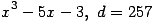
![x^3+x^2-4x-2,\; d=316,\; m=[0, 0, 1; 0, -2, 1; 1, 1, 1] ...(308.1)](eqn/klein-polyhedra_eqn_308_1.png)
![x^3+x^2-4x-1,\; d=321,\; m=[0, -1, 1; -1, 1, 0; 1, 0, -2] ...(320.1)](eqn/klein-polyhedra_eqn_320_1.png)


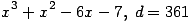
![x^3-x^2-5x-1,\; d=404,\; m=[0, 1, 1; 1, 2, 1; 1, 1, -1] ...(357.1)](eqn/klein-polyhedra_eqn_357_1.png)
![x^3+x^2-5x-4,\; d=469,\; m=[0, 2, 1; 2, 0, 0; 1, 0, -1] ...(368.1)](eqn/klein-polyhedra_eqn_368_1.png)
![x^3-5x-1,\; d=473,\; m=[-1, 1, 1; 1, 2, 0; 1, 0, -1] ...(379.1)](eqn/klein-polyhedra_eqn_379_1.png)
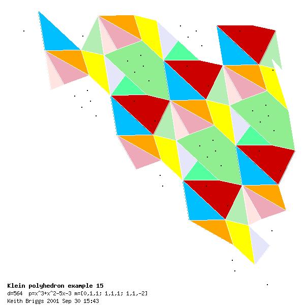
![x^3+x^2-5x-3,\; d=564,\; m=[0, 1, 1; 1, 1, 1; 1, 1, -2] ...(390.1)](eqn/klein-polyhedra_eqn_390_1.png)
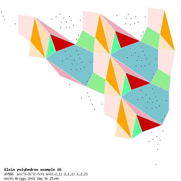
![x^3-3x^2-7x+1,\; d=568,\; m=[0, 2, 1; 2, 1, 2; 1, 2, 2] ...(404.1)](eqn/klein-polyhedra_eqn_404_1.png)
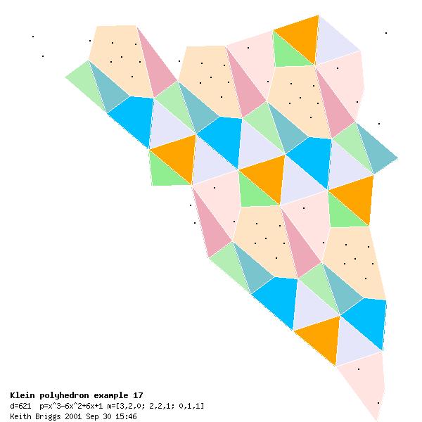
![x^3-6x^2+6x+1,\; d=621,\; m=[3, 2, 0; 2, 2, 1; 0, 1, 1] ...(415.1)](eqn/klein-polyhedra_eqn_415_1.png)

![x^3+x^2-16x-5,\; d=697,\; m=[1,3,2; 3,0,-1; 2,-1,-2] ...(427.1)](eqn/klein-polyhedra_eqn_427_1.png)
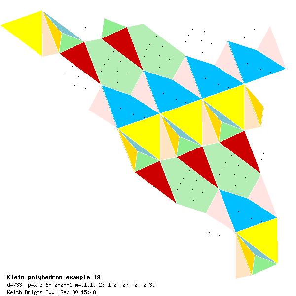
![x^3+x^2-7x-8,\; d=733,\; m=[1,1,-2;1,2,-2;-2,-2,3] ...(439.1)](eqn/klein-polyhedra_eqn_439_1.png)
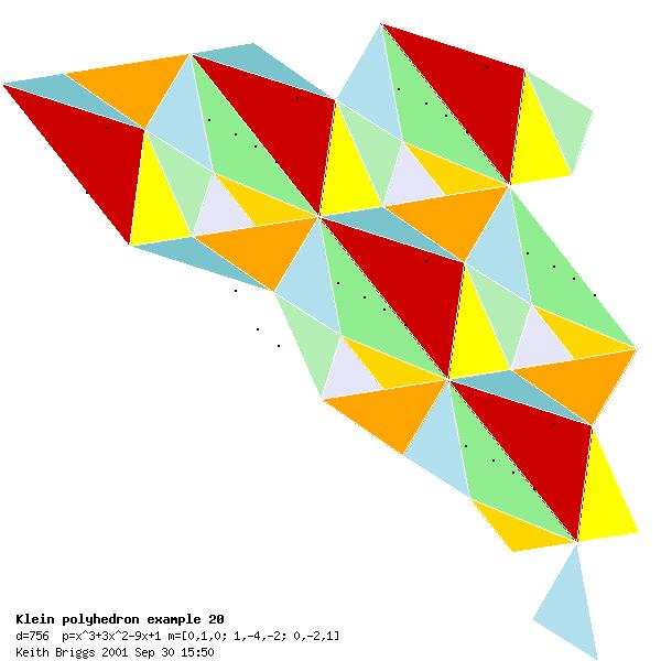
![x^3+3x^2-9x+1,\; d=756,\; m=[0,1,0; 1,-4,-2; 0,-2,1] ...(451.1)](eqn/klein-polyhedra_eqn_451_1.png)

![x^3+2x^2-5x-1,\; d=785,\; m=[2,3,2; 3,-1,-1; 2,-1,-1] ...(475.1)](eqn/klein-polyhedra_eqn_475_1.png)
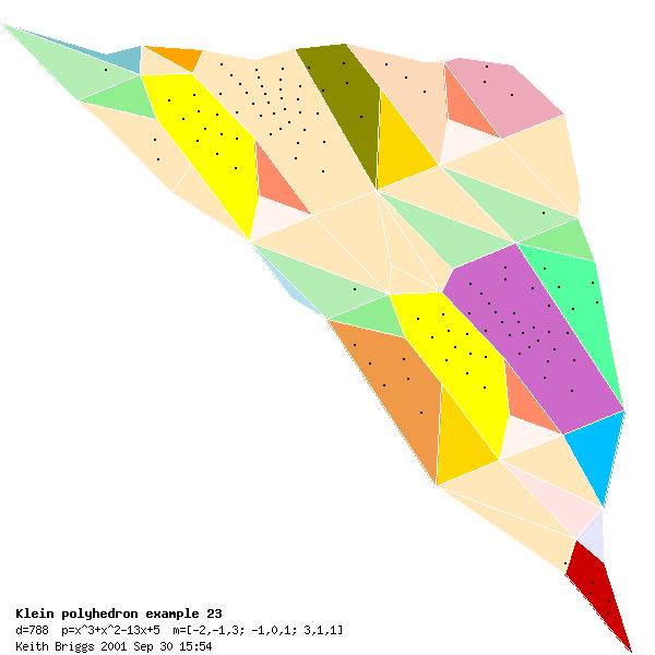
![x^3-x^2-7x-3,\; d=788,\; m=[-2,-1,3; -1,0,1; 3,1,1] ...(487.1)](eqn/klein-polyhedra_eqn_487_1.png)

![x^3-6x-1,\; d=837,\; m=[1,2,1; 2,-1,0; 1,0,0] ...(499.1)](eqn/klein-polyhedra_eqn_499_1.png)