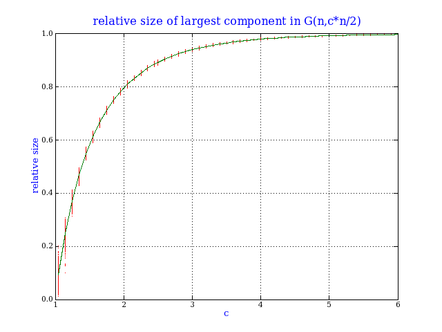
Graph theory and Lambert's W function

The purpose of these notes is to point out two lesser-known applications of Lambert's W function occurring implicitly in two areas of graph theory.

Lambert's W function is defined as the inverse of the map w→w*exp(w) on the interval (-1/e,∞). I use the principal branch, defined as the greater value if there are two inverses (which happens on (-1/e,0)). See the mathworld article for more details. See here for programs to compute W.

Recall the well-known result concerning rooted labelled trees: -W(-z) has a Taylor expansion with coefficients n^n-1/n!, in which the term n^n-1 enumerates rooted labelled trees on n nodes. This result is combinatorial; by contrast the two applications of W below are analytic. Below, G(n,m) is the random graph model in which there are n nodes and m edges distributed uniformly and independently, and G{n,p} is the random graph model in which there are n nodes and each possible edge appears independently with probability p.

The random graph phase transition

See B. Bollabás, Modern graph theory, page 241. Bollabás shows that in the random graph G(n,cn/2) on n nodes, with c>1, the relative size L(1)/n of the largest component satisfies |L(1)/n - γ| < ω/sqrt(n) for almost every graph (as n→∞), where γ is given as the solution of e^-cγ=1-γ. Here ω is the size of the largest clique.

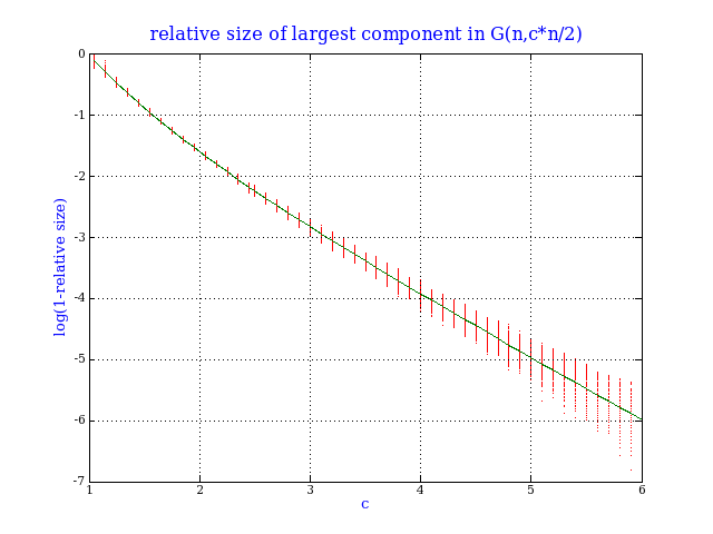
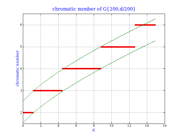
Here is a simulation to verify this. For each value of c, I generated 1000 random graphs of 10,000 nodes, and computed the size of the largest component (red dots). The green line is given by γ(c). This is the famous `birth of the giant component'. Note the larger variance near c=1, a typical phase transition behaviour.

Note that for c near 1, we have γ(c)=2(c-1)-8(c-1)²/3+...; and for c near ∞, we have γ(c)=1-exp(-c)-c*exp(-2c)+.... The next plot confirms this large c behaviour.

The two possible values of the chromatic number

See D. Achlioptas & A. Naor, The two possible values of the chromatic number of a random graph Annals of Mathematics, 162 (2005) (available here). The authors show that for fixed d with probability 1 as n→∞, the chromatic number of G{n,d/n} is either k or k+1, where k is the smallest integer such that d < 2klog(k).

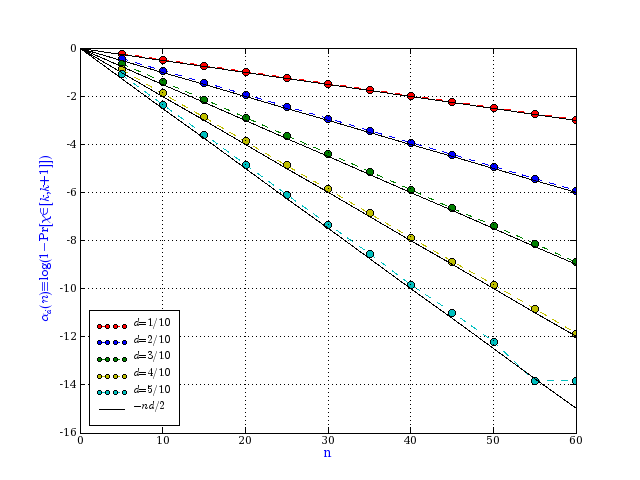
Here is a simulation to verify this. For each value of d, I generated 10 random graphs each of 200 nodes, and computed the exact chromatic number (red dots). The green lines are given by d/(2W(d/2))+1/2 and d/(2W(d/2))+3/2.

We can go further and look at the rate of approach to probability 1. The next graph (each point is the average of 1 million trials) suggests that for small d, we have Prob[χ ∈ [k,k+1]] ≈ 1-exp(-dn/2). As far as I know, this conjecture is unproven.